SVMs & Autoencoders
Comprehensive implementation of Support Vector Machines and Deep Autoencoders for image classification and dimensionality reduction on CIFAR-10 and MNIST datasets, built from scratch using NumPy, CuPy, and PyTorch.
github.com/pompos02/NeuralNetworks-DeepLearningProject Overview
This project consists of two major assignments demonstrating the implementation of classical machine learning algorithms and modern deep learning approaches. Assignment 2 focuses on Support Vector Machines with different kernels and optimization techniques, while Assignment 3 explores autoencoders for dimensionality reduction and image reconstruction.
- Assignment 2: SVM implementations using primal form with gradient descent, dual form with kernel methods, and Sequential Minimal Optimization (SMO)
- Assignment 3: Autoencoder architectures for MNIST digit reconstruction, with comparison to PCA and classification performance analysis
- All implementations built from scratch using NumPy and CuPy for GPU acceleration
- Comprehensive hyperparameter tuning and performance evaluation with 150+ visualization figures
Assignment 2: Support Vector Machines
Implementation of SVM algorithms from scratch for binary classification of CIFAR-10 dataset (cats vs dogs), using only NumPy and CuPy.
1. Linear SVM with Primal Form
Implemented using Hinge Loss with L2 regularization and Stochastic Gradient Descent optimization. Features include GPU acceleration with CuPy, learning rate scheduling, standardization, and data augmentation.
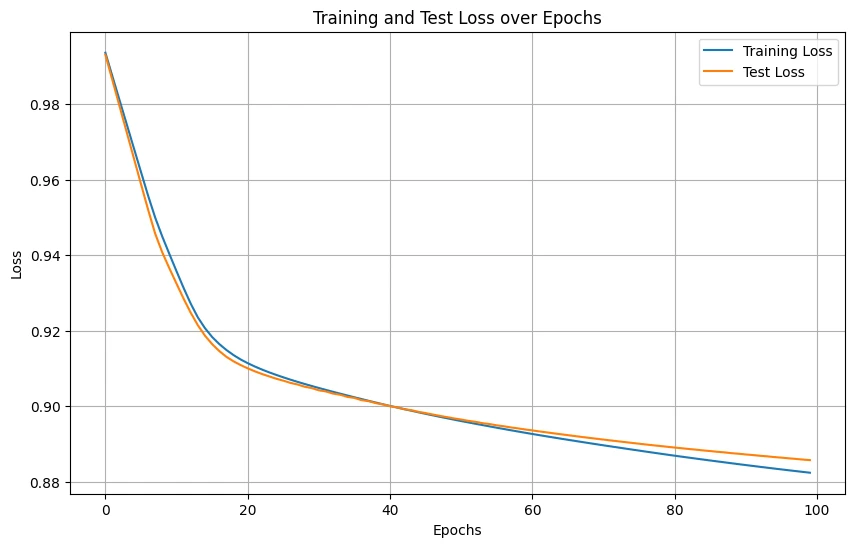
Initial Linear SVM results showing training progress and confusion matrix
Performance Optimization Results:
| Configuration | Train Acc | Test Acc |
|---|---|---|
| Basic Implementation | 59.06% | 58.55% |
| With LR Scheduler | 56.74% | 56.60% |
| + Data Augmentation | 60.53% | 60.55% |
| Final Optimized | 63.69% | 63.40% |
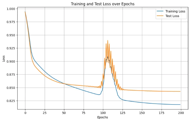
Final optimized Linear SVM with hyperparameter tuning
2. Polynomial SVM with Dual Form
Using polynomial kernel K(x,y) = (x·y + c)^d, implemented in dual form with gradient ascent optimization.
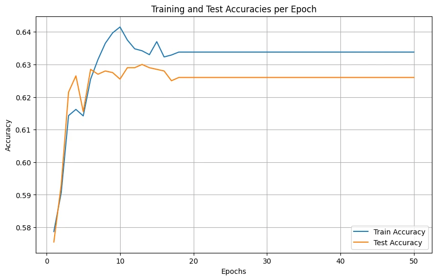
Performance by Configuration:
| Hyperparameters | Train Acc | Test Acc |
|---|---|---|
| Degree=3, C=3.0 | 63.38% | 62.60% |
| Best: Degree=2, C=10 (with tuning) | 73.49% | 64.25% |
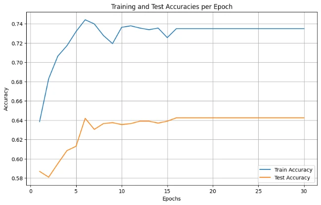
Comprehensive grid search results showing optimal hyperparameter combinations
3. RBF SVM with Sequential Minimal Optimization
Using RBF kernel K(x,y) = exp(-γ||x-y||²) with SMO algorithm for efficient training. Achieved the best overall performance among all SVM variants.
SMO Algorithm Performance:
| Implementation | Train Acc | Test Acc | Time |
|---|---|---|---|
| RBF SMO (Optimized) | 89.91% | 65.70% | 102 mins |
| RBF SMO (Basic) | 68.54% | 64.25% | Long |
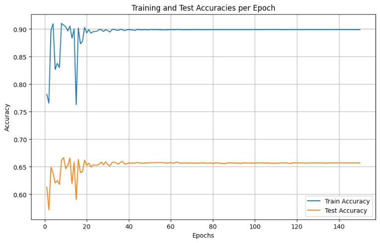
RBF SVM training curves showing convergence and final performance metrics
Assignment 3: Autoencoders & Deep Learning
Implementation and comparison of autoencoder architectures for MNIST digit reconstruction, with evaluation against PCA and classification performance analysis using a CNN.
Autoencoder Architectures
1. Basic Autoencoder
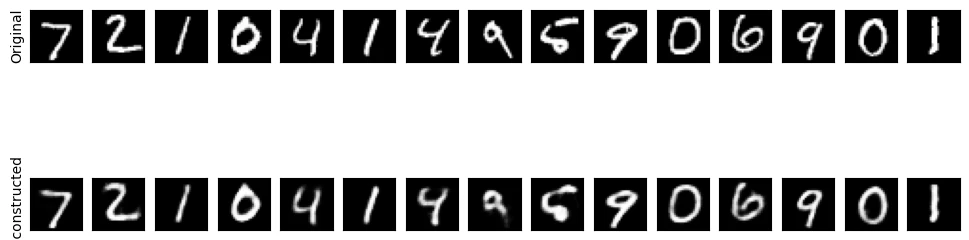
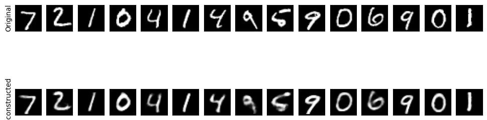
Architecture: 784 → 128 → 32 → 128 → 784 with ReLU activation (hidden) and Sigmoid (output). Trained using MSE loss.
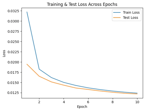
Results: Train Loss: 0.0103, Test Loss: 0.0099
Basic Autoencoder training loss progression
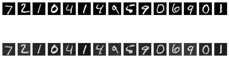
Sample digit reconstructions from Basic Autoencoder
2. Deep Autoencoder
Enhanced architecture: 784 → 512 → 256 → 64 → 256 → 512 → 784 with deeper layers for better feature learning.
Improved Results: Train Loss: 0.0045, Test Loss: 0.0047 (50% reduction in MSE)
Deep Autoencoder showing superior convergence and lower loss
Latent Space Analysis
t-SNE visualization of the 32D and 64D latent spaces reduced to 2D, showing clear digit clustering patterns.
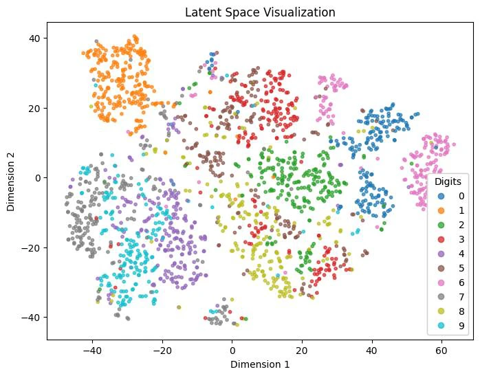
t-SNE visualization showing distinct digit clusters in latent space
Reconstruction Quality Comparison
Comparison of Methods:
| Method | Test MSE | Bottleneck Size |
|---|---|---|
| Deep Autoencoder | 0.0047 | 64 |
| Basic Autoencoder (64) | 0.0063 | 64 |
| PCA Reconstruction | 0.0090 | 64 |
Side-by-side comparison of PCA and Autoencoder reconstructions
CNN Classification Network
Implemented a CNN to classify MNIST digits using three different inputs: original data, autoencoder reconstructions, and PCA reconstructions.
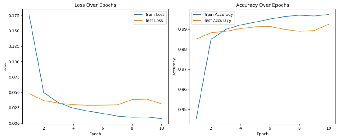
CNN training and validation accuracy/loss curves showing excellent convergence
Classification Performance:
| Input Type | CNN Accuracy | Performance Drop |
|---|---|---|
| Original MNIST | 98.89% | Baseline |
| Deep AE Reconstruction | 98.27% | -0.62% |
| PCA Reconstruction | 98.22% | -0.67% |
Per-Digit Analysis
Analysis of reconstruction error by digit class reveals which digits are most challenging for the models.
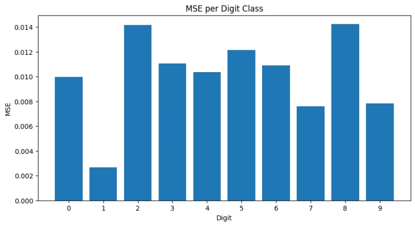
Basic Autoencoder per-digit loss
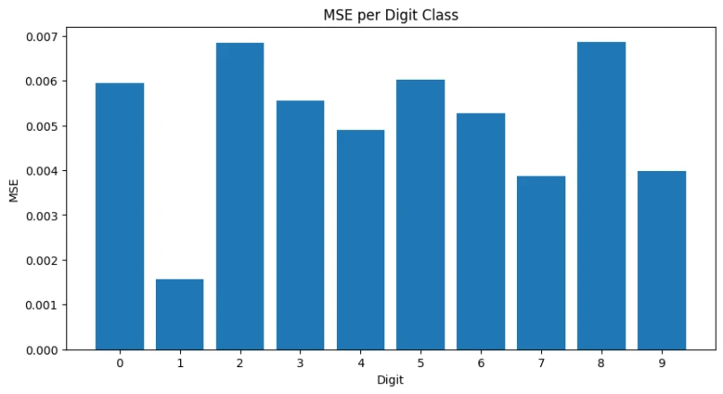
Deep Autoencoder per-digit performance
Key Findings:
- Best Reconstructed: Digit 1 (0.001576 MSE) - Simple linear structure
- Most Challenging: Digit 8 (0.006864 MSE) - Complex loops and overlapping regions
- Consistent Pattern: Digits 0, 2, 5, 8 show higher reconstruction error across all models
Technical Implementation
High-Performance Computing
- GPU Acceleration: CuPy integration achieving 100x speedup for SVM training
- Efficient Memory Management: Batch processing and vectorized operations
- PyTorch Integration: Automatic differentiation and GPU support for deep learning
Advanced Optimization Techniques
- Learning Rate Scheduling: Up-then-down adaptive strategies
- Regularization: L2 penalty, dropout, early stopping
- Data Augmentation: Horizontal flip, random crop
- Standardization: Z-score normalization for faster convergence
Key Results Summary
SVM Performance (CIFAR-10 Cats vs Dogs)
| Algorithm | Test Accuracy | Complexity |
|---|---|---|
| RBF SVM (SMO) | 65.70% | High |
| Polynomial SVM | 64.25% | Medium |
| Linear SVM | 63.40% | Low |
| Linear SMO | 61.90% | Medium |
| K-NN (k=1) | 57.85% | Low |
Autoencoder & CNN Results (MNIST)
| Model | Metric | Performance |
|---|---|---|
| CNN on Original | Accuracy | 98.89% |
| Deep Autoencoder | MSE Loss | 0.0047 |
| Basic Autoencoder | MSE Loss | 0.0099 |
| PCA (64 components) | MSE Loss | 0.0090 |
| CNN on Deep AE Reconstruction | Accuracy | 98.27% |
| CNN on PCA Reconstruction | Accuracy | 98.22% |
Key Insights
1. Architecture Impact
Deeper autoencoders significantly outperform shallow ones (50% MSE reduction). Non-linear mappings (autoencoders) superior to linear methods (PCA) for complex image reconstruction.
2. Classification Robustness
Minimal accuracy drop (<1%) when classifying reconstructed images demonstrates excellent information preservation across all methods.
3. Computational Trade-offs
RBF SVM achieves highest accuracy (65.70%) but requires extensive training time (102+ minutes). Linear methods provide excellent baseline performance with fast training.
4. Method Complementarity
Classical methods (PCA, Linear SVM) provide interpretable and fast baselines. Modern methods (Deep AE, RBF SVM) achieve superior performance with increased complexity.
Technical Stack
Core Libraries
- NumPy & CuPy for GPU-accelerated computing
- PyTorch for deep learning implementations
- scikit-learn for baseline comparisons
- Matplotlib & Seaborn for visualizations
Datasets
- CIFAR-10: 60,000 RGB images, 32x32 pixels, 10 categories
- MNIST: 70,000 grayscale digit images, 28x28 pixels
- Binary classification: cats vs dogs
- 10-class digit recognition