Demand Forecasting in Retail
Comprehensive research exploring machine learning models for predicting retail demand using the M5 Competition Dataset from Walmart, featuring hierarchical forecasting and deep learning approaches.
github.com/pompos02/M5-CompetitionDemandForecastingOverview
This project, based on my thesis "Demand Forecasting in Retail", investigates multiple forecasting approaches ranging from traditional statistical methods to deep learning models. The research addresses the critical business challenge of inventory management and demand prediction across hierarchical sales data.
The project leverages the M5-Competition Dataset, one of the most comprehensive real-world retail forecasting challenges, featuring 42,840 hierarchical time series from Walmart stores across the United States spanning over 5 years of daily sales data.
Dataset Characteristics
Core Statistics:
- 42,840 hierarchical time series from Walmart stores
- 1,969 days of daily sales data (January 2011 - June 2016)
- 3,049 individual products across 3 categories and 7 departments
- 10 stores spanning 3 states (California, Texas, Wisconsin)
- Rich contextual data: pricing, calendar events, SNAP eligibility
Hierarchical Structure:
The dataset enables analysis at 12 aggregation levels:
- Total sales (1 series)
- State level (3 series)
- Store level (10 series)
- Category and Department levels
- Product-Store combinations (30,490 series)
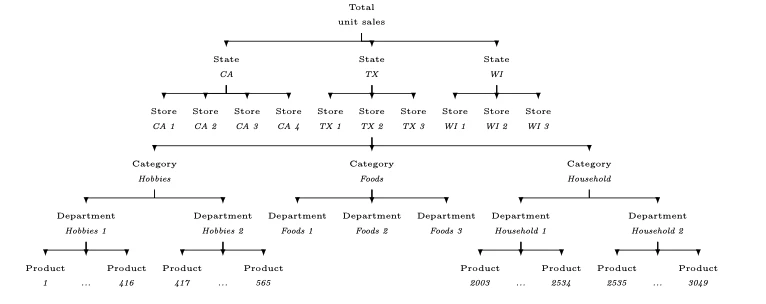
Figure: M5 Dataset hierarchical structure showing organization from total sales down to individual product-store combinations
Technical Stack
- Data Processing: pandas, NumPy (handling ~3GB raw data expanding to ~15GB after feature engineering)
- Machine Learning: scikit-learn, LightGBM
- Deep Learning: PyTorch, PyTorch Lightning, Darts (time series library)
- Statistical Models: statsmodels (for Exponential Smoothing)
- Visualization: Matplotlib, Seaborn
Data Exploration Insights
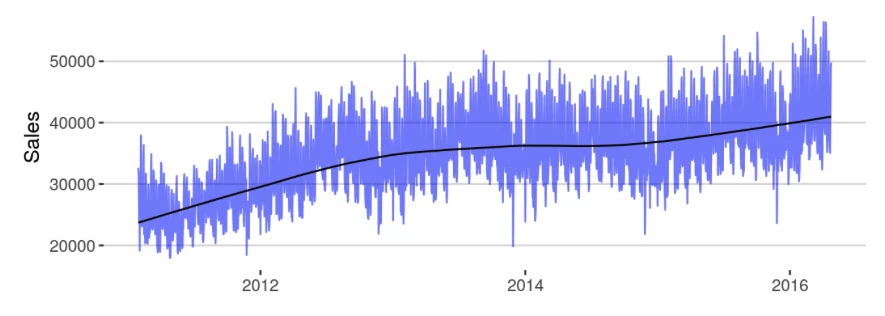
Overall Sales Patterns:
- Clear upward trend with seasonal variations and weekly cyclicality
- Notable sales drops on Christmas Day due to store closures
- Strong annual cyclicality with holiday peaks
- Consistent weekend sales dominance
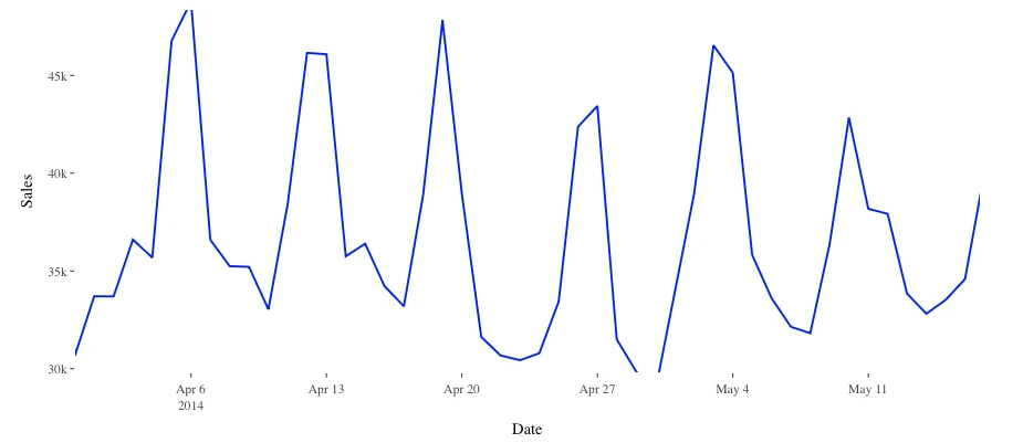
Figure: Overall sales trends showing clear upward trajectory with seasonal patterns
Geographic Distribution:
- California accounts for ~45% of total sales with notable drops in 2013 and 2015
- Texas shows ~35% of sales with more stable patterns
- Wisconsin exhibits ~20% with significant seasonal variations
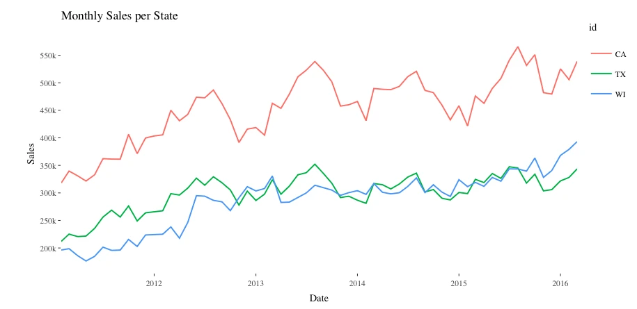
Figure: Sales comparison across states showing California's dominance in sales volume
Product Category Performance:
- FOODS category dominates (65% of sales) with consistent weekly seasonality
- HOUSEHOLD (20%) shows strong promotional sensitivity
- HOBBIES (15%) exhibits high seasonality and event-driven spikes
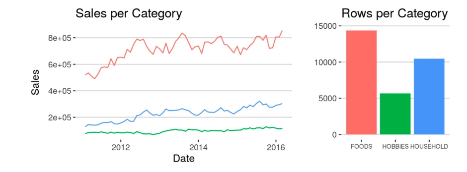
Figure: Product category comparison showing FOODS as the dominant category
Store-Level Analysis:
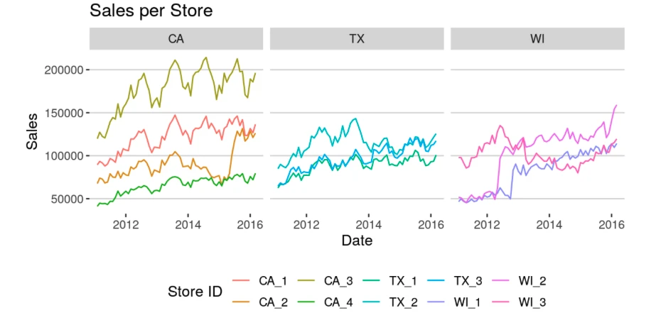
Figure: Individual store performance showing significant variations within and across states
Department-Level Patterns:
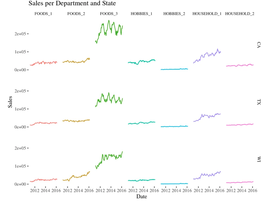
Figure: Sales patterns across departments showing FOODS_3 dominance
Seasonality Analysis:
- Annual peaks: November-December (40-60% sales increase)
- Low periods: January-February post-holiday decline
- Weekend dominance: 20-30% higher sales than weekdays
- State-specific patterns: Wisconsin shows inverted seasonal trends
Annual seasonal patterns
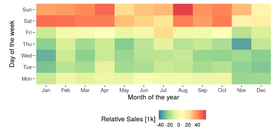
Weekly patterns showing weekend dominance
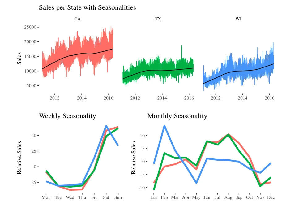
Figure: State-specific seasonal patterns after trend removal and scaling
Comprehensive Feature Engineering
Price-Based Features:
- Current selling price and historical statistics (min, max, mean, std)
- Price momentum indicators (weekly, monthly, annual trends)
- Price volatility measures and normalization
- Cross-product price relationships
Temporal Features:
- Calendar features: Day of month, week, month, year, day of week
- Holiday and event markers (religious, cultural, sporting events)
- Weekend indicators and seasonal decomposition
Statistical Features:
- Rolling window statistics: 7, 14, 28-day moving averages
- Lag features: Sales history from 1, 7, 14, 21, 28 days prior
- Exponentially weighted moving averages
- Trend indicators using first differences
Models Implemented
1. Linear Regression
Baseline statistical approach using 28-day lag features
- Simple interpretable model for benchmark comparison
- Utilizes engineered features from preprocessing pipeline
2. Exponential Smoothing
Holt-Winters method with additive seasonality
- 7-day seasonal period capturing weekly patterns
- Individual models per product-store combination
- No external features - pure time series approach
- Excellent computational efficiency
3. LightGBM (Three Architectures)
Gradient boosted decision trees at multiple aggregation levels:
- Item-Store Level: Individual models per product-store combination
- Category-Store Level: Multivariate models per category-store (28 models per horizon)
- Store Level: Comprehensive models per store handling all products
- Feature-rich approach incorporating all engineered features
4. LSTM Neural Network
Global deep learning model with advanced architecture:
- 4 hidden layers with 128 neurons each
- 28-day input window predicting next 7 days
- Single model trained on all time series
- MinMax scaling (0-1) applied per time series
- Selected features: price, temporal, and statistical indicators
Feature Importance Analysis
Random Forest Analysis:
- Price features (mean, std) show highest importance scores
- Temporal index critical for capturing seasonality
- Product variety (item_nunique) impacts store demand significantly
- Price momentum (monthly/yearly trends) highly informative
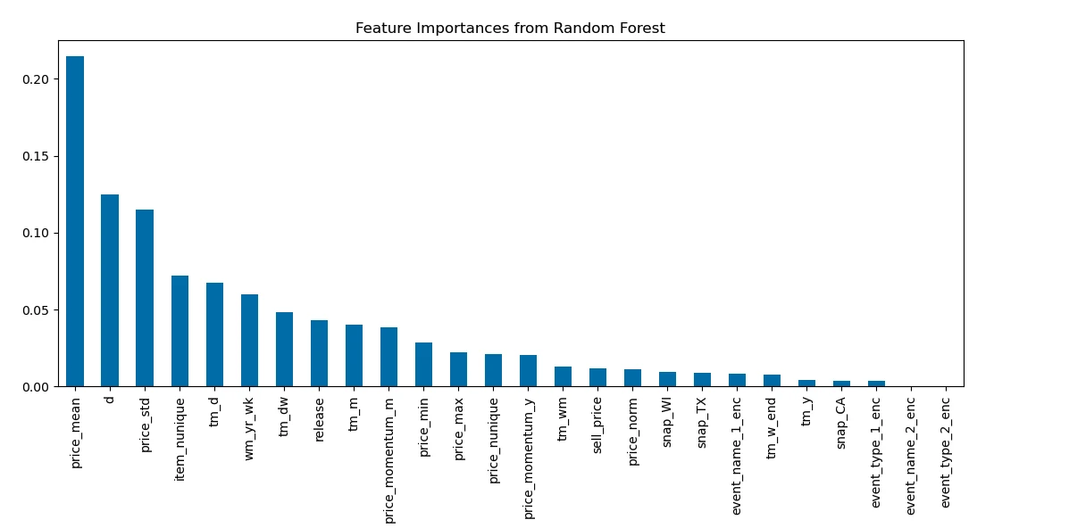
Figure: Random Forest feature importance showing price and temporal features as key predictors
Mutual Information Analysis:
- Captures non-linear relationships missed by correlation
- All price-related variables show high mutual information
- Different features provide unique complementary information
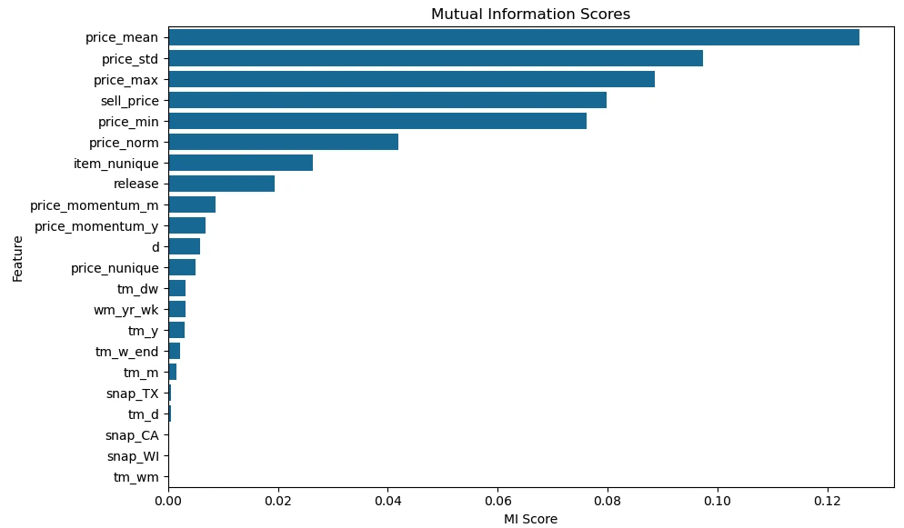
Figure: Mutual Information analysis highlighting non-linear relationships between features and sales
SHAP Analysis (LightGBM):
- Recent sales history (lag-1) shows highest impact
- Feature significance decreases with temporal distance
- Product-specific characteristics (item_id) contribute substantially
- Multiple features work together for optimal predictions
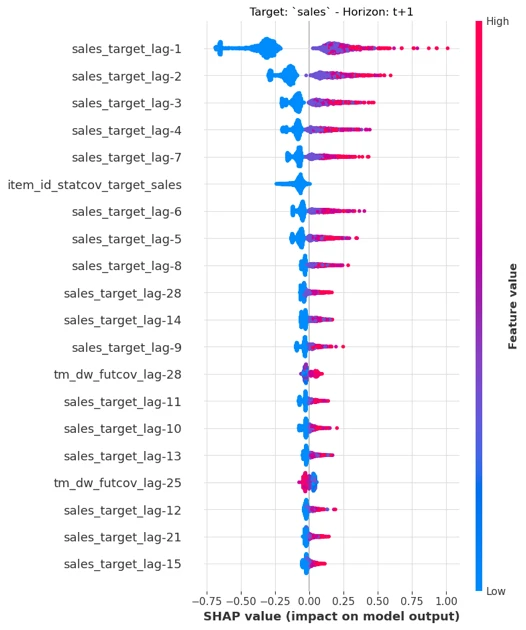
Figure: SHAP analysis revealing feature contribution patterns for one-step-ahead sales prediction
Performance Results
Overall Model Comparison:
| Model | MAE | RMSE | WRMSSE | Rank |
|---|---|---|---|---|
| LSTM | 1.14 | 1.43 | 0.884 | 1st |
| Exp. Smoothing | 1.11 | 1.44 | 0.888 | 2nd |
| LGBM-store | 1.17 | 1.46 | 0.894 | 3rd |
| LGBM-category | 1.14 | 1.46 | 0.898 | 4th |
| Linear Regression | 1.14 | 1.47 | 0.914 | 5th |
| LGBM-item | 1.22 | 1.57 | 0.957 | 6th |
Key Findings:
- LSTM Excellence: Best WRMSSE (0.884) - would rank 11th in M5 competition (only 0.009 points from winner)
- Exponential Smoothing Surprise: Best MAE (1.11) despite simplicity - would achieve 23rd place in M5
- Store-Level LGBM: Best balance among LGBM variants
- Item-Level Challenges: Insufficient data per model led to poor generalization
Error Distribution Analysis
RMSE Distribution:
- All models show strong concentration of RMSE values in 0-1 range
- LSTM demonstrates most consistent error distribution with lowest outlier counts (267 cases with RMSE > 10)
- LGBM-item exhibits highest maximum RMSE (~120) indicating severe overfitting cases
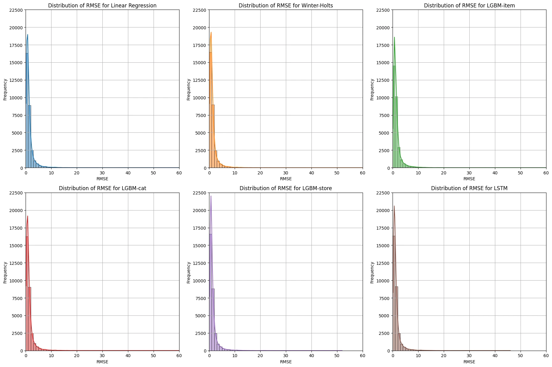
RMSE distribution across models
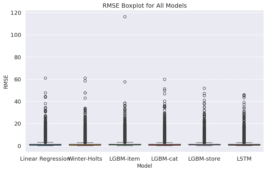
BoxPlot revealing model stability
MAE Distribution:
- MAE distributions show smoother patterns than RMSE with reduced outlier impact
- Median performance similar across models, but variance differs significantly
- Less sensitivity to outliers compared to RMSE
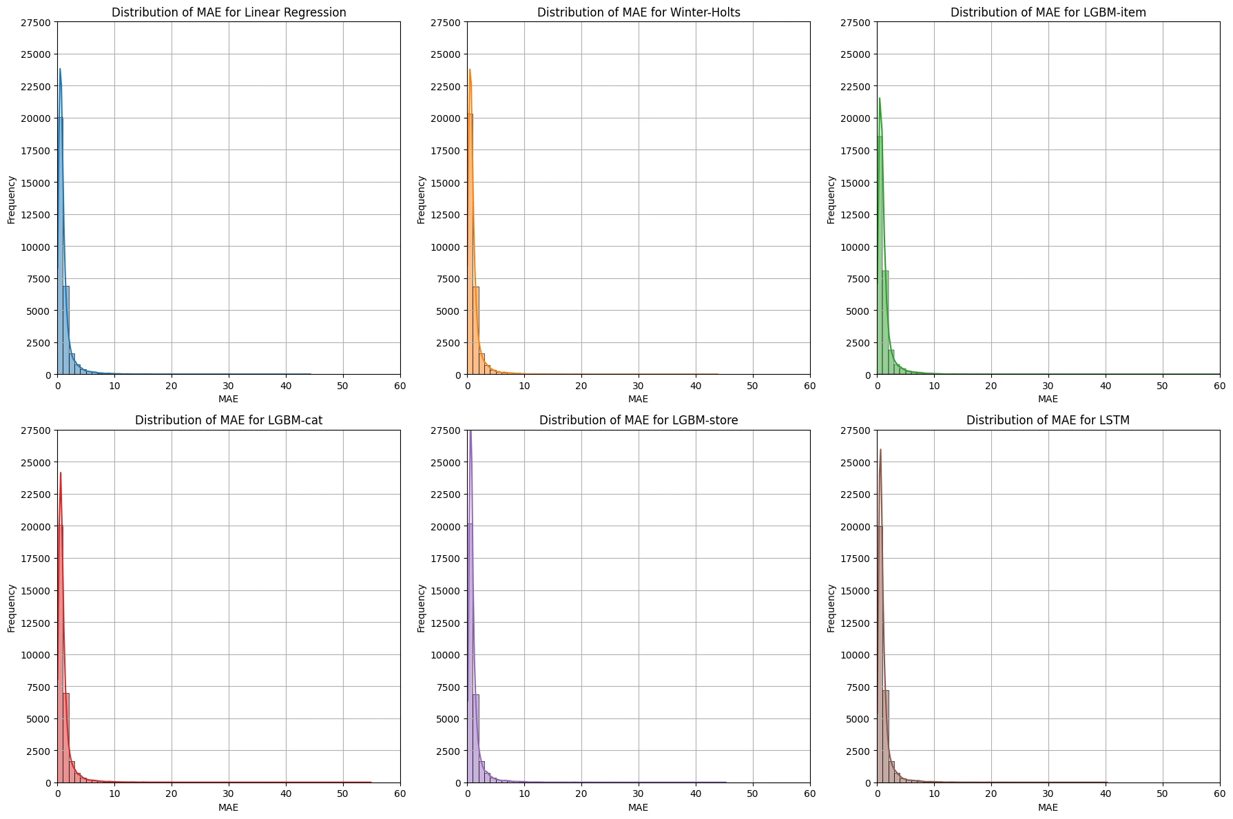
MAE distribution patterns
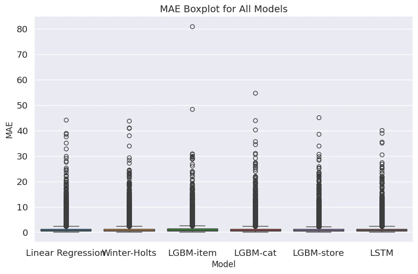
MAE BoxPlot comparison
Category-Specific Performance
Outstanding Performance:
- CA_1 HOUSEHOLD: RMSE = 1.03 (excellent accuracy)
- CA_1 HOBBIES: RMSE = 1.26 (strong performance)
- Texas stores: Consistent performance across all categories
Challenging Categories:
- CA_3 FOODS: RMSE = 2.50 (highest error due to high purchase frequency variability)
- WI_2 FOODS: RMSE = 1.74 (seasonal pattern complexity)
- FOODS category generally more difficult than HOUSEHOLD/HOBBIES
Conclusion
This comprehensive study demonstrates that deep learning approaches (LSTM) achieve superior overall performance for retail demand forecasting, approaching top M5 competition results. However, traditional methods like Exponential Smoothing remain highly competitive with significant advantages in computational efficiency and interpretability.
The research provides practical guidance for model selection based on specific business contexts, balancing accuracy requirements, computational constraints, and interpretability needs. The achieved results validate the effectiveness of the implemented methodology and provide valuable insights for real-world retail forecasting applications.